Summary of AlexNet Paper

Alexnet is a deep neural network which learns visual knowledge from images to classify a given image. It had produced breakthrough results in ImageNet LSVRC-2010 contest achieving a top-1 error rate of 37.5 % which was better than previous start of art methods which achieved 47.1%. The network consists of 8 layers out of which 5 were convolutional layers and other 3 were fully connected layers. The below Section details its architecture

Architecture

For ILSVRC-2010, it was trained on 1.2 million images, validated on 50,000 images and tested on 150,000 images

Layer 1

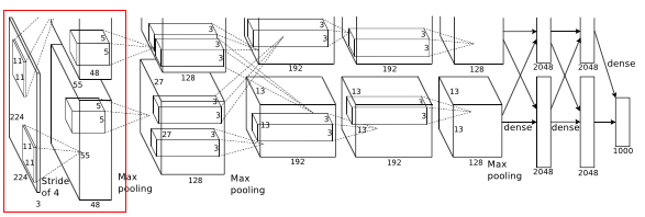
Before image(s) is given to this layer, variable resolution images in training set are re-scaled to a fixed size of 256 * 256 as deep neural networks expects all inputs to be of fixed size. This is done by first rescaling the image such that shorter side is of length 256, and then central 256*256 is cropped out.

To prevent overfitting the training images on this net, dropout of 0.5 in some layers and two methods of data augmentation where labels are preserved were used. One is in which random 224 * 224 patches(and their horizontal reflections) were extracted from each image. Thus this method increase the size of training set by reasonable amount. Another is to perform a transformation to vary the intensity and color of illumination for a image as object identity is invariant to these images.

And Rectified Linear unit neurons are used, where its activation function is max(0,x). By using these neurons, training time will be decreased according to the observations.

• Then this 224 * 224 * 3 image is given to 1st convolutional layer.
• Where this layer filters the image with 96 kernels of size 11 * 11 * 3
• Stride - 4, assuming padding is 2 Here stride(s) < kernel size(z) (4 < 11), so this overlapping pooling. According to the paper, the models with overlapping pooling find it slightly more difficult to overfit.
• Therefore output = (224 - 11 + 2 *2)/4 + 1 = 55
• Output is of size 55 * 55 * 96
• To this output, local response normalization(LRN) is applied which is a brightness normalization.
• After LRN, max pooling layer is applied where stride is 2 and kernel size is 3 * 3
• Therefore now output is 27((55 - 3)/2 + 1 ) * 27 * 96

Layer 2

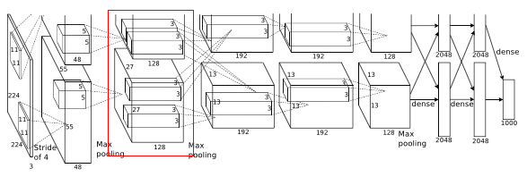
• Input to this layer is 27 * 27 * 96
• Filters = 256
• Kernel size = 5 * 5 * 48, padding = 2
• Stride = 1
• Output width or height = (27 - 5 + 2 * 2)/1 + 1 = 27
• Output is 27 * 27 * 256
• This is followed by LRN and max pooling layer
• Final output layer is
  • Max pooling kernel of size 3 * 3 and stride 1
  • Output width or height = (27 - 3 + 2)/1 + 1 = 27
  • Final output = 27 * 27 * 256

Layer 3

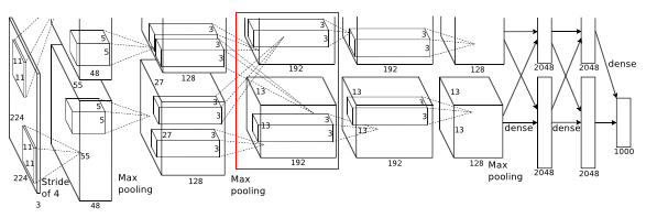
• Input to this layer is 27 * 27 * 256
• Filters = 384
• Kernel size 3 * 3 *256, padding - 1
• Output width or height = (27 - 3 + 2)/1 + 1 = 27
• Final output is 27 * 27 * 384

Layer 4

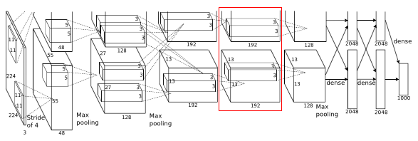
• Input to this layer is 27 * 27 * 384
• Filters = 384
• Kernel size is 3 * 3 * 192, padding = 1
• Output width or height = (27 - 3 + 2)/1 + 1 = 27
• Final output is 27 * 27 * 384

Layer 5

Similarly after the fifth convolutional layer

• As filters = 256
• Output is 27 * 27 * 256
• After the max pooling layer
  • Kernel size is 3 * 3 and stride 2
  • Final output width or height = (27 - 3 )/2 + 1 = 13
  • Final output is 13 * 13 * 256 And other two layers are fully connected layers of 4096 each

Softmax

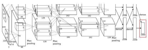
To the final layer 1000 way softmax is used to get predicted probabilities for each class.