Summary of Fast R-CNN Paper

Paper

• Title: Fast R-CNN (fastRCNN)
• Submission date: 30 Apr 2015

Key Contributions

• This paper proposes a Fast Region-based Convolutional Network model (Fast R-CNN) for object detection.
• Fast R-CNN uses a streamlined training process with one fine-tuning rather than multi-stage training process used by R-CNN.
• Compared to previous R-CNN network, Fast R-CNN employs several innovations to improve training and testing speed while also increasing detection accuracy.

Achievements

• Fast R-CNN trains the very deep VGG16 network $9 \times$ faster than R-CNN, is $213 \times$ faster at test-time, and achieves a higher mAP on PASCAL VOC 2012.
• Compared to SPPnet, Fast R-CNN trains VGG16 $3 \times$ faster, tests $10 \times$ faster, and is more accurate.

Fast R-CNN

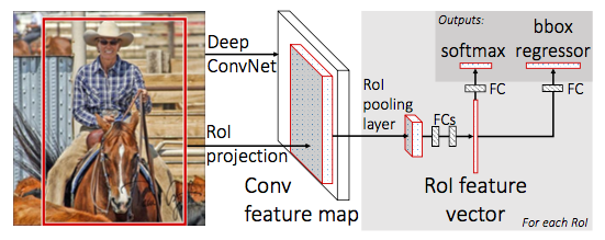
The above figure illustrates Fast R-CNN architecture. Similar to the R-CNN, category independent region or object proposals are extracted from the image. Then Fast R-CNN network takes entire input image and a set of object proposals. The network first processes the whole image with several convolutional and max pooling layers to produce a conv feature map. Then, for each object proposal a region of interest (ROI) pooling layer extracts a fixed length feature vector from the feature map. Then each feature vector is fed into a sequence of fully connected (fc) layers.

While training Fast R-CNN, authors initialized the architecture with the pre-trained networks. The initialized pre-trained networks undergoes the following transformations.

• The ROI pooling layer replacing the last max pooling layer
• The network’s last fully connected layer and softmax are replaced with the two sibling layers i.e. a fully connected layer with softmax over K + 1 categories (no of categories plus background) and category-specific bounding box regressors.
• The network is modified to take two inputs: a list of images and a list of RoIs in those images.

Large fully connected layer can be made faster by using truncated SVDs. In object detection, nearly half of the time is spent computing in fully connected layers. Therefore SVDs are used for the speed-up of networks.

Experiments

The experiments use the following ImageNet models

• S (Small): AlexNet Model
• M (Medium): VGG_CNN_M_1024, which has the same depth as S but is wider.
• L (Large): Very deep VGG16 model.

In experiments authors compared Fast RCNN against the other top methods available at that time. They tested the network on the three datasets: VOC07, VOC 2010 and VOC 2012. All the experiments of Fast RCNN use single-scale training and testing.

From the results, we observed that SPPnet uses five scales during both training and testing. The improvement of Fast R-CNN over SPPnet illustrates that even though Fast R-CNN uses single-scale training and testing, fine-tuning the conv layers provides a large improvement in mAP (mean average precision (%)).

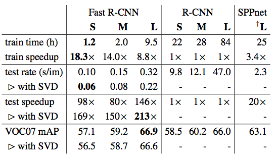
The above table shows runtime comparision between same models in Fast R-CNN, R-CNN and SPPnet. Fast R-CNN, R-CNN uses single-scale mode. SPPnet uses the multi-scale training, i.e. five scales.

Conclusion

The following main results from experiments supports the paper contributions

• State-of-the-art mAP on VOC07, 2010 and 2012
• Fast training and testing compared to R-CNN, SPPnet
• Fine-tuning conv layers in VGG 16 improves mAP