on
Summary of R-CNN Paper
Paper
- Title: Rich feature hierarchies for accurate object detection and semantic segmentation (R-CNN)
- Submission date: 11 Nov 2013
- This paper is very long and does not have typical division of sections like architecture, training and experiments. Everything is explained together in two sections: object detection and semantic segmentation.
Key Contributions
- This network aims to get better performance on object detection as well as semantic segmentation.
- Developed an approach that combines two key insights:
- To apply high-capacity convolutional neural networks (CNNs) to bottom-up region proposals in order to localize and segment objects.
- When labeled training data is scarce, supervised pre-training for an auxiliary task, followed by domain-specific fine tuning, yields a significant performance boost.
- In this paper, authors answered the question “To what extent do the CNN classification results on ImageNet generalize to object detection results on the PASCAL VOC Challenge?”
- This paper is the first to show that a CNN can lead to dramatically higher object detection performance on PASCAL VOC.
R-CNN
This network is named as R-CNN becuase it combines region proposals with CNNs. Therefore R-CNN is Regions with CNN features. Unlike image classification, detection and segmentation requires localizing objects within a image. CNN localization problem is solved by operating within the “recognition using regions”.
Object detection
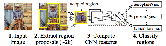
R-CNN object detection system consists of three modules.
- The first module generates category-independent region proposals.
- The second module is a large convolutional neural network that extracts a fixed-length feature vector from each region.
- The third module is a set of class specific linear SVMs.
Authors pre-trained the CNN on a large auxiliary dataset (ILSVRC2012 classification). Then they adapted this CNN for the object detection and the new domain. Then the developed R-CNN are tested on VOC 2010-2012, ILSVRC2013 datasets.
| VOC 2010 test | mAP |
|---|---|
| DPM v5 | 33.4 |
| UVA | 35.1 |
| Regionlets | 39.7 |
| SegDPM | 40.4 |
| R-CNN | 50.2 |
| R-CNN BB | 53.7 |
The above table presents detection average precision (%) on VOC 2010 test. R-CNN BB is R-CNN combined with Bounding-box regression (BB). These methods are compared to the other base line methods like DPM v5, UVA, Regionlets and SegDPM. R-CNN, UVA and Regionlets use selective search region proposals. DPM and SegDPM use context rescoring which is not used by other methods.
The following table compares R-CNN to the entries in the ILSVRC2013 competition and to the post-competition OverFeat result. OverFeat uses a sliding-window CNN for detection. Methods preceeded by * use outside training data.
| ILSVRC2013 test | mAP |
|---|---|
| *R-CNN BB | 31.4 |
| *OverFeat | 24.3 |
| UvA-Euvision | 22.6 |
| *NEC-MU | 20.9 |
| Toronto A | 11.5 |
| SYSU_Vision | 10.5 |
| GPU_UCLA | 9.8 |
| Delta | 6.1 |
| UIUC-IFP | 1 |
Semantic segmentation
Then leading semantic segmentation system called $O_{2}P$, “second-order pooling”. $O_{2}P$ uses CPMC to generate 150 region proposals per image and then predicts the quality of each region, for each class, using support vector regression (SVM). Using the same framework, the following three strategies are defined. All of these strategies begin by warping the rectangular window around the region to $227 \times 227$.
- The full R-CNN ignores the region’s shape and computes CNN features directly on the warped window
- The fg R-CNN computes CNN features only on a region’s foreground mask.
- The full+fg R-CNN simply concatenates the full and fg features.
| full R-CNN | fg R-CNN | full+fg R-CNN | ||||
|---|---|---|---|---|---|---|
| $O_{2}P$ | $fc_6$ | $fc_7$ | $fc_6$ | $fc_7$ | $fc_6$ | $fc_7$ |
| 46.4 | 43.0 | 42.5 | 43.7 | 42.1 | 47.9 | 45.8 |
The above table shows segmentation mean accuracy (%) on VOC 2011 validation, which explains R-CNN network against $O_{2}P$. $fc_6$ and $fc_7$ are the last two fully connected layers in the R-CNN network. From above, we can observe that $fc_6$ always outperforms $fc_7$.
The following table presents results on the VOC 2011 test set, comparing our best-performing method, $fc_6$ (full+fg) against two strong baselines - the “Regions and Parts” (R&P) and $O_{2}P$ methods. Without any fine-tuning, R-CNN outperforms two strong baselines.
| VOC 2011 test | mean |
|---|---|
| R&P | 40.8 |
| $O_{2}P$ | 47.6 |
| full+fg R-CNN $fc_{6}$ | 47.9 |
Conclusion
The then best performing systems were complex ensemblems combining multiple low-level image features with high-level context from object detectors and scene classifiers. Whereas this paper presented a simple and scalable object detection algorithm that combines tools from computer vision and deep learning. The prposed method gave a 30% relative improvement over the best previous results on PASCAL VOC 2012.