on
Summary of Densenet Paper
Paper
- Title: Densely Connected Convolutional Networks (Densenet)
- Submission date: 25 Aug 2016
Key Contributions
- Developed densenet model for image classification.
- The idea of the dense convolutional neural network is to connect each layer to every other layer in the feed forward fashion.
- Concatenating feature-maps learned by different layers increases variation in the input of subsequent layers and improves efficiency.
Advantages
The advantages of the denset are:
- Decrease the vanishing-gradient problem
- Improve feature propogation both in forward as well as backward fashion
- Encourage the feature reuse
- Reducing the number of parameters
Densenet
Increased in the depth of convolutional neural network caused a problem of vanishing information about the input or gradiant when passing through many layers. In order to solve this, authors introduced an architecture with simple connectivity pattern to ensure the maximum flow of information between layers both in forward computation as well as in backward gradiants computation. This network connects all layers in such a way each layer obtains additional inputs from all preceding layers and passes its own feature-maps to all subsequent layers.
The network comprises L layers. Each layer implements a non-linear transformation $H_l([x_0, x_1, …, x_{l-1}])$ where l indexes the layer. $H_l(.)$ can be a composite function of operations such as Batch normalization (BN), rectified linear unit (ReLU), pooling or convolution (Conv). Here $[x_0, x_1, …, x_{l-1}]$ refers to concatenation of the feature-maps produced in layers $0,…,l-1$.
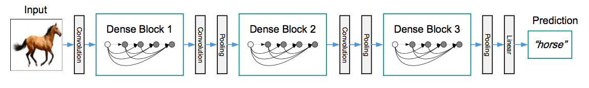
The concatenation operation mentioned above is not vitable when the size of feature-maps are variable. As we know, the essential part of image recognition convolutional networks is down-sampling layers. To facilitate the down-sampling in the architecture, authors divided the entire architecture into multiple densely connected dense blocks. The layers between these dense blocks are transition layers which perform convolution and pooling.
DenseNet vs ResNet
Superficially, DenseNets are quite similar to ResNets. But the inputs format is different in two networks which lead to substantially different behaviours. The following table presents the differences between two networks.
| Feature | Densenet | Resnet |
|---|---|---|
| Format of passing previous layer features to other layers | by concatening | by summation |
| No of inputs to $l^{th}$ layer | $l$ | $1$ |
| Total no of connections in L-layer network | $L(L+1)/2$ | $L$ |
| The way to address vanishing-gradient problem | using dense connections | using stochastic depth |
| Performance Improvement | using power of deep architecture | using power of feature reuse |
Experiments
Experiments are done on popular datasets like CIFAR-10 (C10), CIFAR-100 (C100), SVHN and Imagenet datasets. In C10+ and C100+ datasets, “+” indicates data augmentation. Error rates (%) on validation data are presented in the below table. The k parameter in DenseNet (k=<num>) below is growth rate, which means each composite function of a DenseNet produces k feature-maps.
| Method | Depth | Params | C10 | C10+ | C100 | C100+ | SVHN |
|---|---|---|---|---|---|---|---|
| ResNet | 110 | 1.7M | 13.63 | 6.41 | 44.74 | 27.22 | 2.01 |
| ResNet + Stochiastic Depth | 110 | 1.7M | 11.66 | 5.23 | 37.80 | 24.58 | 1.75 |
| ResNet + Stochiastic Depth | 1202 | 10.2M | - | 4.91 | - | - | - |
| ResNet (pre-activation) | 164 | 1.7M | 11.26 | 5.46 | 35.58 | 24.33 | - |
| ResNet (pre-activation) | 1001 | 10.2M | 10.56 | 4.62 | 33.47 | 22.71 | - |
| DenseNet (k=12) | 40 | 1.0M | 7.00 | 5.24 | 27.55 | 24.42 | 1.79 |
| DenseNet (k=12) | 100 | 7.0M | 5.77 | 4.10 | 23.79 | 20.20 | 1.67 |
| DenseNet (k=24) | 100 | 27.2M | 5.83 | 3.74 | 23.42 | 19.25 | 1.59 |
| Densenet-BC (k=12) | 100 | 0.8M | 5.92 | 4.51 | 24.15 | 22.27 | 1.76 |
| Densenet-BC (k=24) | 250 | 15.3M | 5.19 | 3.62 | 19.64 | 17.60 | 1.74 |
| Densenet-BC (k=40) | 190 | 25.6M | - | 3.46 | - | 17.18 | - |
- DenseNet-B network - It introduces 1 x 1 convolution as a bottleneck layer before each 3 x 3 layer to reduce the number of input feature-maps, and thus to improve computational efficiency.
- DenseNet-BC network - It is same as DenseNet-B with additional compression factor.
Compression factor $(\theta)$ - If a denseblock generates m feature-maps, then the next transition layer outputs $\theta \times m$ feature-maps (where $\theta$ varies from 0 to 1). This compression factor is introduced to improve model compactness.
In the above experiments, Densenet and DenseNet-BC uses 3 dense blocks as shown in the above network diagram. Whereas for training on Imagenet dataset, DenseNet-BC uses four dense blocks.
| Model | top-1 | top-5 |
|---|---|---|
| DenseNet-BC-121 | 25.02 / 23.61 | 7.71 /6.66 |
| DenseNet-BC-169 | 23.80 / 22.08 | 6.85 / 5.92 |
| DenseNet-BC-201 | 22.58 / 21.46 | 6.34 / 5.54 |
| DenseNet-BC-264 | 22.15 / 20.80 | 6.12 / 5.29 |
The above table shows top-1 and top-5 error rates on the Imagenet validation data set with a single-crop / 10-crop testing.